Zoom Network architectures & practical considerations
Zoom session 2
Time:
11:30 am Pacific Time.
Access:
Same zoom access as in the first session.
Topic:
Introduction to network architectures and implementation constraints/solutions.
Slides
Click below to open the presentation.
Once in the presentation, navigate the slides with the left and right arrows and refresh any page to show the link that will take you back here.

A few notes from the slides
Types of learning
There are now more types of learning than those presented here. But these initial types are interesting because they will already be familiar to you.
Supervised learning
You have been doing supervised machine learning for years without looking at it in the framework of machine learning:
- Regression is a form of supervised learning with continuous outputs
- Classification is supervised learning with discrete outputs
Supervised learning uses training data in the form of example input/output \((x_i, y_i)\) pairs.
Goal:
If \(X\) is the space of inputs and \(Y\) the space of outputs, the goal is to find a function \(h\) so that
for each \(x_i \in X\),
\(h_\theta(x_i)\) is a predictor for the corresponding value \(y_i\)
(\(\theta\) represents the set of parameters of \(h_\theta\)).
→ i.e. we want to find the relationship between inputs and outputs.
Unsupervised learning
Here too, you are familiar with some forms of unsupervised learning that you weren't thinking about in such terms:
Clustering, social network analysis, market segmentation, PCA … are all forms of unsupervised learning.
Unsupervised learning uses unlabelled data (training set of \(x_i\)).
Goal:
Find structure within the data.
Gradient descent

There are several gradient descent methods:
Batch gradient descent uses all examples in each iteration and is thus slow for large datasets (the parameters are adjusted only after all the samples have been processed).
Stochastic gradient descent uses one example in each iteration. It is thus much faster than batch gradient descent (the parameters are adjusted after each example). But it does not allow any vectorization.
Mini-batch gradient descent is an intermediate approach: it uses mini-batch sized examples in each iteration. This allows a vectorized approach (and hence parallelization).
The Adam optimization algorithm is a popular variation of mini-batch gradient descent.
Types of ANN
Fully connected neural networks

Each neuron receives inputs from every neuron of the previous layer and passes its output to every neuron of the next layer.
Convolutional neural networks
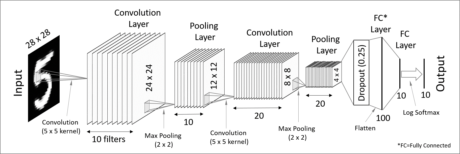
Convolutional neural networks (CNN) are used for spatially structured data (e.g. in image recognition).
Images have huge input sizes and would require a very large number of neurons in a fully connected neural net. In convolutional layers, neurons receive input from a subarea (called local receptive field) of the previous layer. This greatly reduces the number of parameters.
Optionally, pooling (combining the outputs of neurons in a subarea) reduces the data dimensions. The stride then dictates how the subarea is moved across the image. Max-pooling is one of the forms of pooling which uses the maximum for each subarea.
Recurrent neural networks

Recurrent neural networks (RNN) such as Long Short-Term Memory (LSTM) are used for chain structured data (e.g. in speech recognition).
They are not feedforward networks (i.e. networks for which the information moves only in the forward direction without any loop).
Deep neural networks
The first layer of a neural net is the input layer. The last one is the output layer. All the layers in-between are called hidden layers. Shallow neural networks have only one hidden layer and deep networks have two or more hidden layers. When an ANN is deep, we talk about Deep Learning (DL).