Practice Loading and exploring the MNIST
The MNIST dataset
As you learnt in the past 2 videos, the MNIST is one of the classic datasets used for testing machine learning systems. It consists of pairs of images of handwritten digits and their corresponding labels.
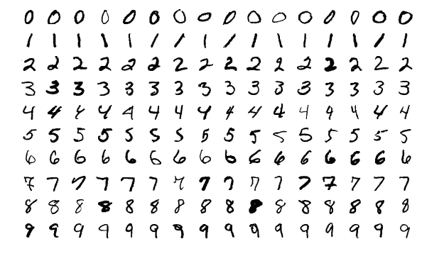
The images are composed of 28x28 pixels of greyscale RGB codes ranging from 0 to 255 and the labels are the digits from 0 to 9 that each image represents.
There are 60,000 training pairs and 10,000 testing pairs.
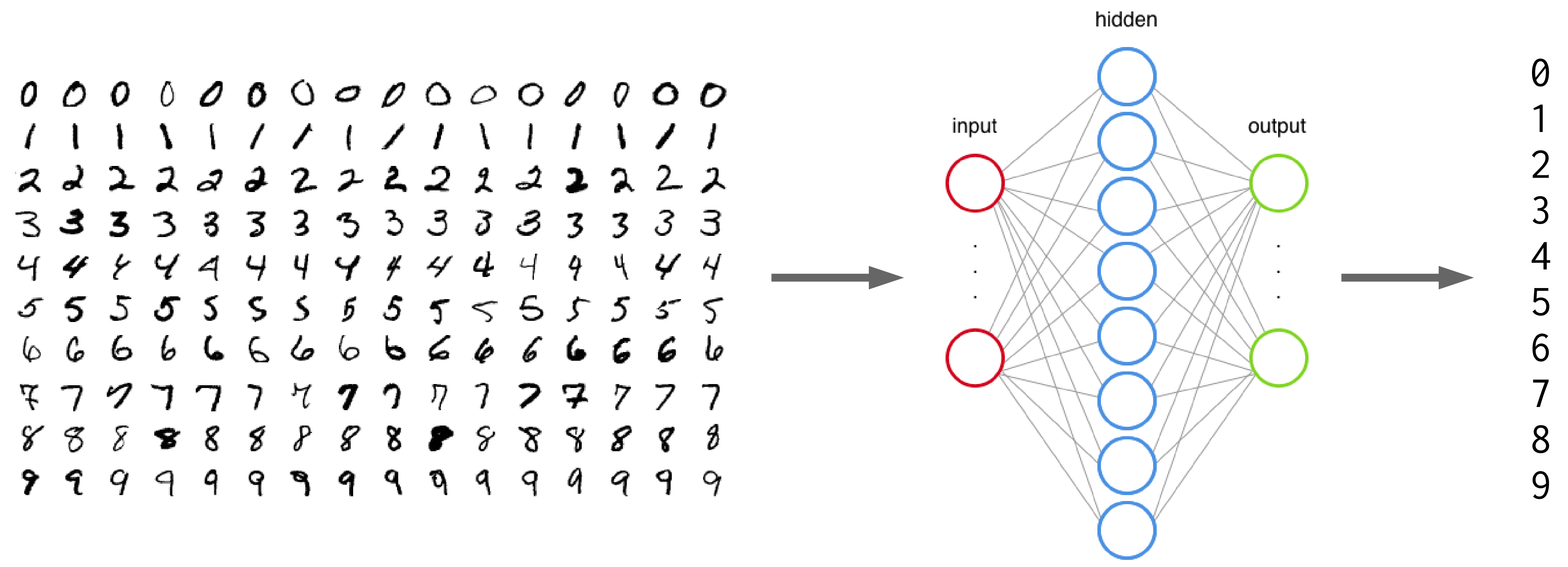
The goal is to build a neural network which can learn from the training set to properly identify the handwritten digits and which will perform well when presented with the testing set that it has never seen. This is a typical case of supervised learning.
Start an interactive job
Before you can start running Python code, you need to source your Python virtual environment and start an interactive job:
$ source ~/env/bin/activate
$ salloc --cpus-per-task=1 --mem=3G --time=0:30:0   # edit as needed
$ python
Load Python modules
from matplotlib import pyplot as plt
import torch
from torchvision import datasets, transforms
Set the device argument to CPU
Since our training cluster does not have GPUs, we are setting the device argument to 'cpu':
device = torch.device('cpu')If you have a CUDA-enabled GPU on your computer and if you are running the code locally, you can run:
device = torch.device('cuda:0')This is also what you will want to use when running jobs on the Compute Canada clusters.
More elegantly, you can write a conditional:
device = torch.device('cuda:0' if torch.cuda.is_available() else 'cpu')Get and prepare the MNIST data
In the Compute Canada clusters, a good place to store data shared amongst users of a project is in the /project file system; more precisely, in /project/def-<group> , where <group> is usually the name of your PI. You can access it from your home through a symbolic link in ~/projects : ~/projects/def-<group> .
In our training cluster, we are all part of the group def-sponsor00 , so we will all download and access the MNIST data in ~/projects/def-sponsor00/data .
You can download the dataset directly from the MNIST website, but the PyTorch package TorchVision has tools to download the classic vision datasets, including the MNIST. This is why we loaded modules from torchvision at the start of this script.
Training data
Now, we will download the MNIST training data, transform it to tensor, and normalize it.
First, let's define a transformation (the mean and standard deviation of the MNIST training data are 0.1307 and 0.3081 respectively, hence these values):
transform = transforms.Compose([
        transforms.ToTensor(),
        transforms.Normalize((0.1307,), (0.3081,))
    ])
Then we can download and transform it:
train_data = datasets.MNIST(
    '~/projects/def-sponsor00/data',
    train=True, download=True, transform=transform)
train=True selects the training set of the MNIST.
Test data
We then do the same with the test data (even though the mean and std of the test data are slightly different, we want to normalize it in the same way):
test_data = datasets.MNIST(
    '~/projects/def-sponsor00/data',
    train=False, transform=transform)
Notice that here, we use train=False to select the test set.
Explore the data
Inspect the data
First, let's check the size of train_data:
print(len(train_data))
OK, that makes sense since the MNIST's training set has 60,000 pairs. train_data has 60,000 elements and we should expect each element to be of size 2 since it is a pair. Let's double-check with the first element:
print(len(train_data[0]))OK. So far, so good. We can print that first pair:
print(train_data[0])And you can see that it is a tuple with:
print(type(train_data[0]))What is that tuple made of?
print(type(train_data[0][0]))
print(type(train_data[0][1]))
It is made of the tensor for the first image (remember that we transformed the images into tensors when we created the objects train_data and test_data) and the integer of the first label (which you can see is 5 when you print train_data[0][1]).
So since train_data[0][0] is the tensor representing the image of the first pair, let's check its size:
print(train_data[0][0].size())That makes sense: a color image would have 3 layers of RGB values (so the size in the first dimension would be 3), but because the MNIST has black and white images, there is a single layer of values—the values of each pixel on a gray scale—so the first dimension has a size of 1. The 2nd and 3rd dimensions correspond to the width and length of the image in pixels, hence 28 and 28.
Run the following:
print(train_data[0][0][0])
print(train_data[0][0][0][0])
print(train_data[0][0][0][0][0])
And think about what each of them represents.
Then explore the test_data
object.
Plot an image from the data
For this, we will use pyplot from matplotlib.
First, we select the image of the first pair and we resize it from 3 to 2 dimensions by removing its dimension of size 1 with torch.squeeze:
img = torch.squeeze(train_data[0][0])
Then, we plot it with pyplot, but since we are in a cluster, instead of showing it to screen with plt.show(), we save it to file:
plt.imshow(img, cmap='gray')
plt.savefig('img.png')
You can now copy the image to your local computer to visualize it. From your local shell:
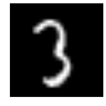
scp userxxx@uu.c3.ca:<path/to/img.png> <path/where/you/want/to/copy/it>This is what that first image looks like:
And indeed, it matches the first label we explored earlier (train_data[0][1]).
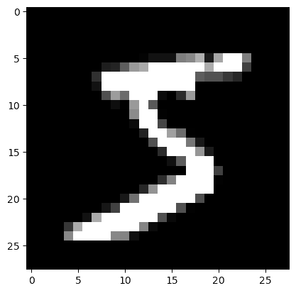
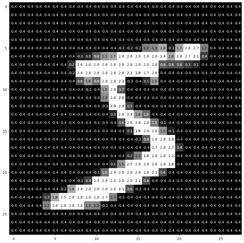
Plot one image with its pixel values
We can plot it with more details by showing the value of each pixel in the image. One little twist is that we need to pick a threshold value below which we print the pixel values in white otherwise they would not be visible (black on near black background). We also round the pixel values to one decimal digit so as not to clutter the result.
imgplot = plt.figure(figsize = (12, 12))
sub = imgplot.add_subplot(111)
sub.imshow(img, cmap='gray')
width, height = img.shape
thresh = img.max() / 2.5
for x in range(width):
    for y in range(height):
        val = round(img[x][y].item(), 1)
        sub.annotate(str(val), xy=(y, x),
                    horizontalalignment='center',
                    verticalalignment='center',
                    color='white' if img[x][y].item() < thresh else 'black')

imgplot.savefig('imgpx.png')
And this is what we get:
Pass the data through DataLoader
PyTorch provides the torch.utils.data.DataLoader class which combines a dataset and an optional sampler and provides an iterable (while training or testing our neural network, we will iterate over that object). It allows, among many other things, to set the batch size and shuffle the data.
So our last step in preparing the data is to pass it through DataLoader.
Training data
train_loader = torch.utils.data.DataLoader(
    train_data, batch_size=20, shuffle=True)
Test data
test_loader = torch.utils.data.DataLoader(
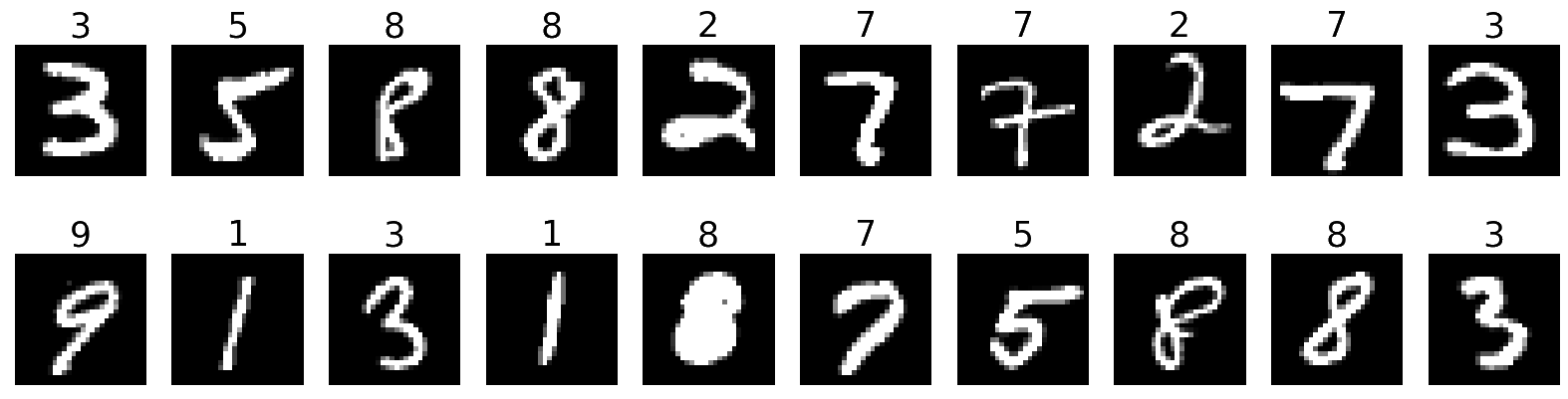
test_data, batch_size=20, shuffle=False)Plot a full batch of images with their labels
Now that we have passed our data through DataLoader, it is easy to select one batch from it. Let's plot an entire batch of images with their labels.
First, we need to get one batch of training images and their labels:
dataiter = iter(train_loader)
batchimg, batchlabel = dataiter.next()
Then, we can plot them:
batchplot = plt.figure(figsize=(20, 5))
for i in torch.arange(20):
    sub = batchplot.add_subplot(2, 10, i+1, xticks=[], yticks=[])
    sub.imshow(torch.squeeze(batchimg[i]), cmap='gray')
    sub.set_title(str(batchlabel[i].item()), fontsize=25)
batchplot.savefig('batchplot.png')
We get:
References
This lesson drew heavily on a model by Muhammad Haseeb.