Reading Concepts
What is machine learning?
Machine learning (ML) can be defined as computer programs whose performance at a task improves with experience.
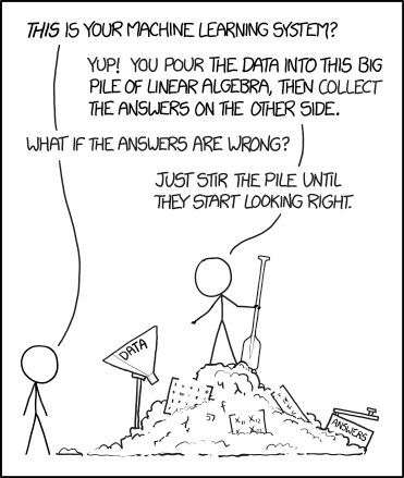
Since this experience comes in the form of data, ML consists of feeding vast amounts of data to algorithms to strengthen pathways.
Example in image recognition
Coding all the possible ways—pixel by pixel—that a picture can represent a certain object is an impossibly large task. By feeding examples of images of that object to a neural network however, we can train it to recognize that object in images that it has never seen (without explicitly programming how it does this!).
Supervised learning
You have been doing supervised machine learning for years without thinking about it in those terms:
- Regression is a form of supervised learning with continuous output
- Classification is supervised learning with discrete output
Supervised learning uses training data in the form of example input/output \((x_i, y_i)\) pairs.
Goal:
If \(X\) is the space of inputs and \(Y\) the space of outputs, the goal is to find a function \(h\) so that
for each \(x_i \in X\), \(h_\theta(x_i)\) is a predictor for the corresponding value \(y_i\)
(\(\theta\) represents the set of parameters of \(h_\theta\)).
→ i.e. we want to find the relationship between inputs and outputs.
Unsupervised learning
Here too, you are familiar with some forms of unsupervised learning that you weren't thinking about in such light:
Clustering, social network analysis, market segmentation, PCA … are all forms of unsupervised learning.
Unsupervised learning uses unlabelled data (training set of \(x_i\)).
Goal:
Find structure within the data.
Artificial neural networks
The next lesson will show you four excellent videos by 3Blue1Brown on neural networks, so you will learn a lot about them then. But in short, artificial neural networks (ANN) are layered networks of units mimicking the concept of biological neurons: inputs are received by every unit, computed, then transmitted to other units. Experience strengthens some connections between units and weakens others.
In biological networks, the information consists of action potentials (neuron membrane rapid depolarizations) propagating through the network. In artificial ones, the information consists of vectors of weights and biases: each unit passes a weighted sum of its input vector with an additional—possibly weighted—bias through an activation function before passing on the output vector to the next layer of units.
Note:
the bias allows to shift the output of the activation function to the right or to the left; it creates an offset.
Schematic of biological neuron:
Schematic of artificial neuron:
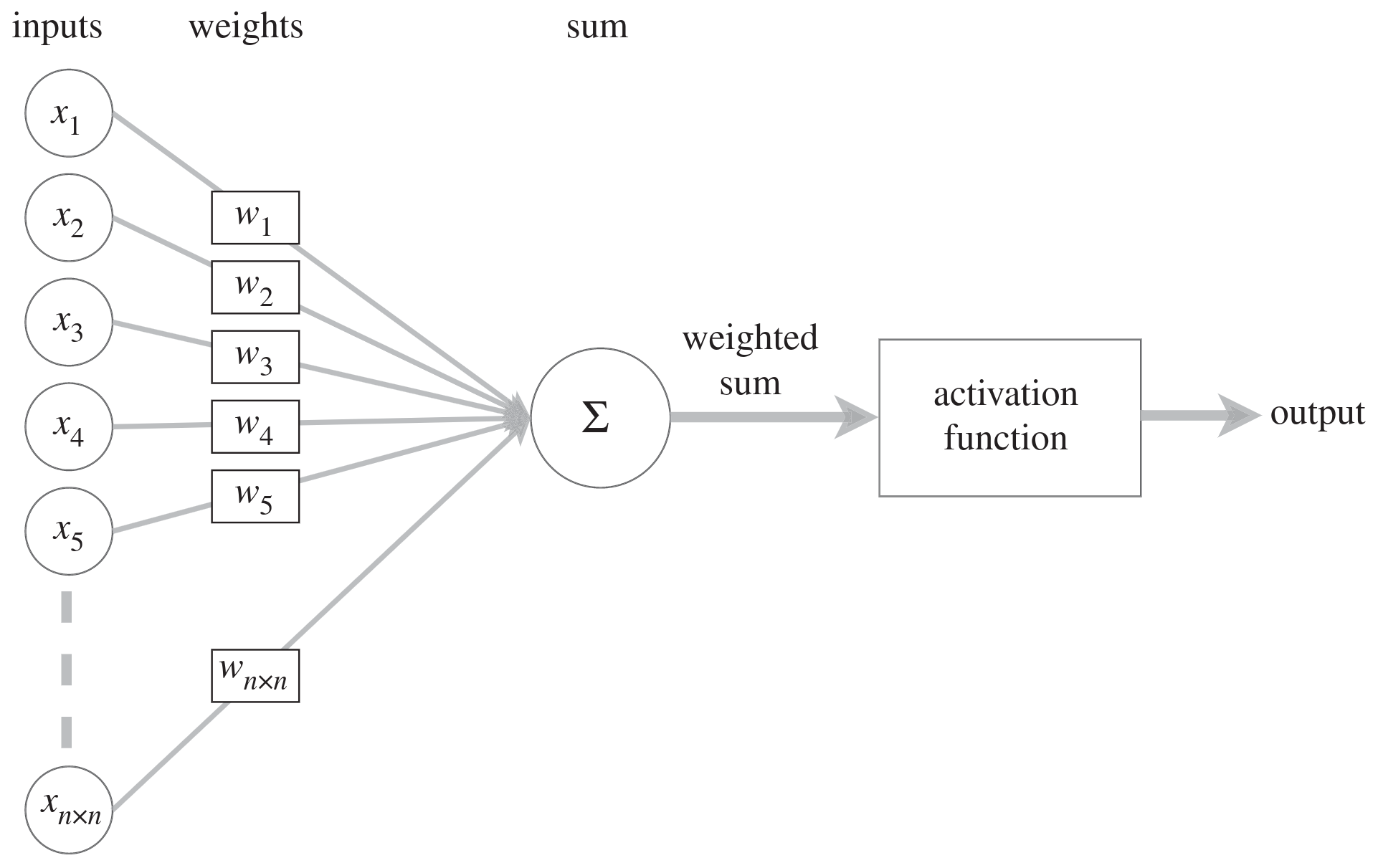
While biological neurons are connected in intricate ways, artificial ones follow a layered structure. Another difference in complexity is in the number of units: the human brain has 65–90 billion neurons. ANN have much fewer units.
Neurons in mouse cortex:
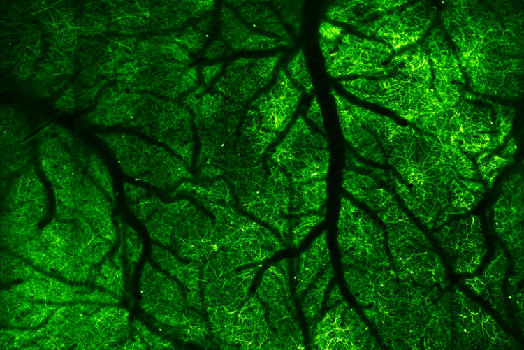
image by Na Ji, UC Berkeley
Neural network with 2 hidden layers:
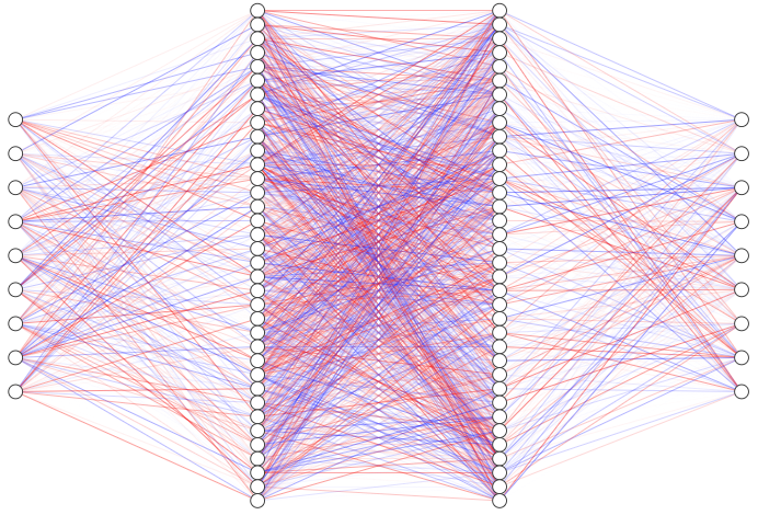
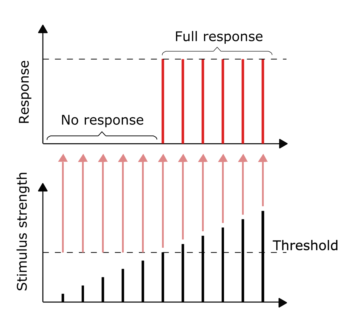
The information in biological neurons is an all-or-nothing electrochemical pulse or action potential. Greater stimuli don’t produce stronger signals but increase firing frequency. In contrast, artificial neurons pass the computation of their inputs through an activation function and the output can take any of the values possible with that function.
Threshold potential in biological neurons:
Some of the most common activation functions in artificial neurons:
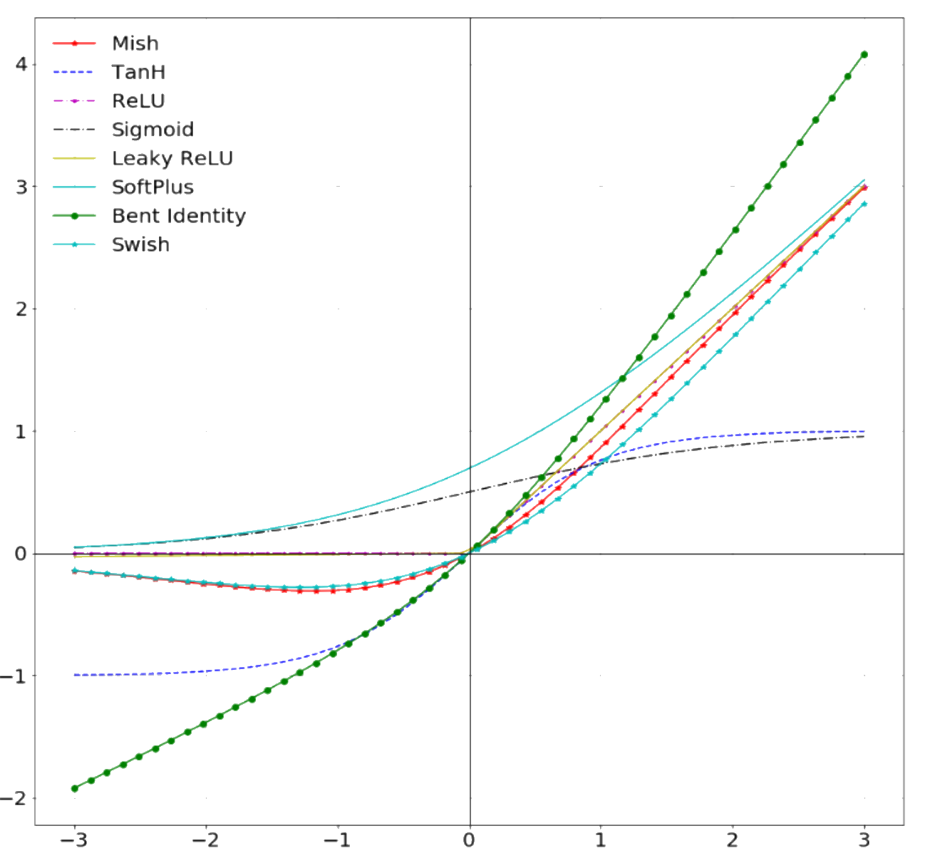
Which activation function to use depends on the type of problem and the available computing budget. Some early functions have fallen out of use while new ones have emerged (e.g. sigmoid got replaced by ReLU which is easier to train).
Learning:
The process of learning in biological NN happens through neuron death or growth and through the creation or loss of synaptic connections between neurons. In ANN, learning happens through optimization algorithms such as gradient descent which minimize cross entropy loss functions by adjusting the weights and biases connecting each layer of neurons over many iterations (cross entropy is the difference between the predicted and real distributions).
Gradient descent:
There are several gradient descent methods:
Batch gradient descent uses all examples in each iteration and is thus slow for large datasets (the parameters are adjusted only after all the samples have been processed).
Stochastic gradient descent uses one example in each iteration. It is thus much faster than batch gradient descent (the parameters are adjusted after each example). But it does not allow any vectorization.
Mini-batch gradient descent is an intermediate approach: it uses mini-batch sized examples in each iteration. This allows a vectorized approach (and hence parallelization).
The Adam optimization algorithm is a popular variation of mini-batch gradient descent.
Types of ANN
Fully connected neural networks
Each neuron receives input from every neuron of the previous layer.
Convolutional neural network
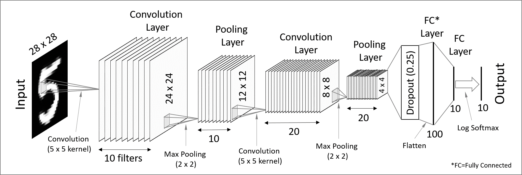
CNN are used for spatially structured data (e.g. image recognition).
Images have huge input sizes and would require a very large number of neurons in a fully connected neural net. In convolutional layers, neurons receive input from a subarea (local receptive field) of the previous layer. This greatly reduces the number of parameters.
Optionally, pooling (combining the outputs of neurons in a subarea) reduces the data dimensions. The stride then dictates how the subarea is moved across the image. Max-pooling is one of the forms of pooling which uses the maximum for each subarea.
Recurrent neural network
RNN (e.g. Long Short-Term Memory or LSTM) are used for chain structured data (e.g. speech recognition).
They are not feedforward networks (i.e. networks for which the information moves only in one direction without any loop).
A bit of vocabulary
- feature: measurable property of a phenomenon
- feature vector: set of a phenomenon's features
- linear predictor function: linear function of a set of coefficients and explanatory variables
- linear classifier: linear predictor function using a feature vector to test whether a phenomenon belongs to a certain class
- perceptron: a type of linear classifier for supervised learning. It is the simplest version of a neural network with a single-layer network mapping a set of inputs to an output thanks to a generalized variation of a linear function
We talk about Deep Learning whenever an ANN consists of 2 or more hidden layers (deep network). Shallow networks only have one hidden layer.

Overfitting
Overfitting—extracting noise from the data while it does not represent general meaningful structure and has no predictive power—is a common problem when developing ML models.
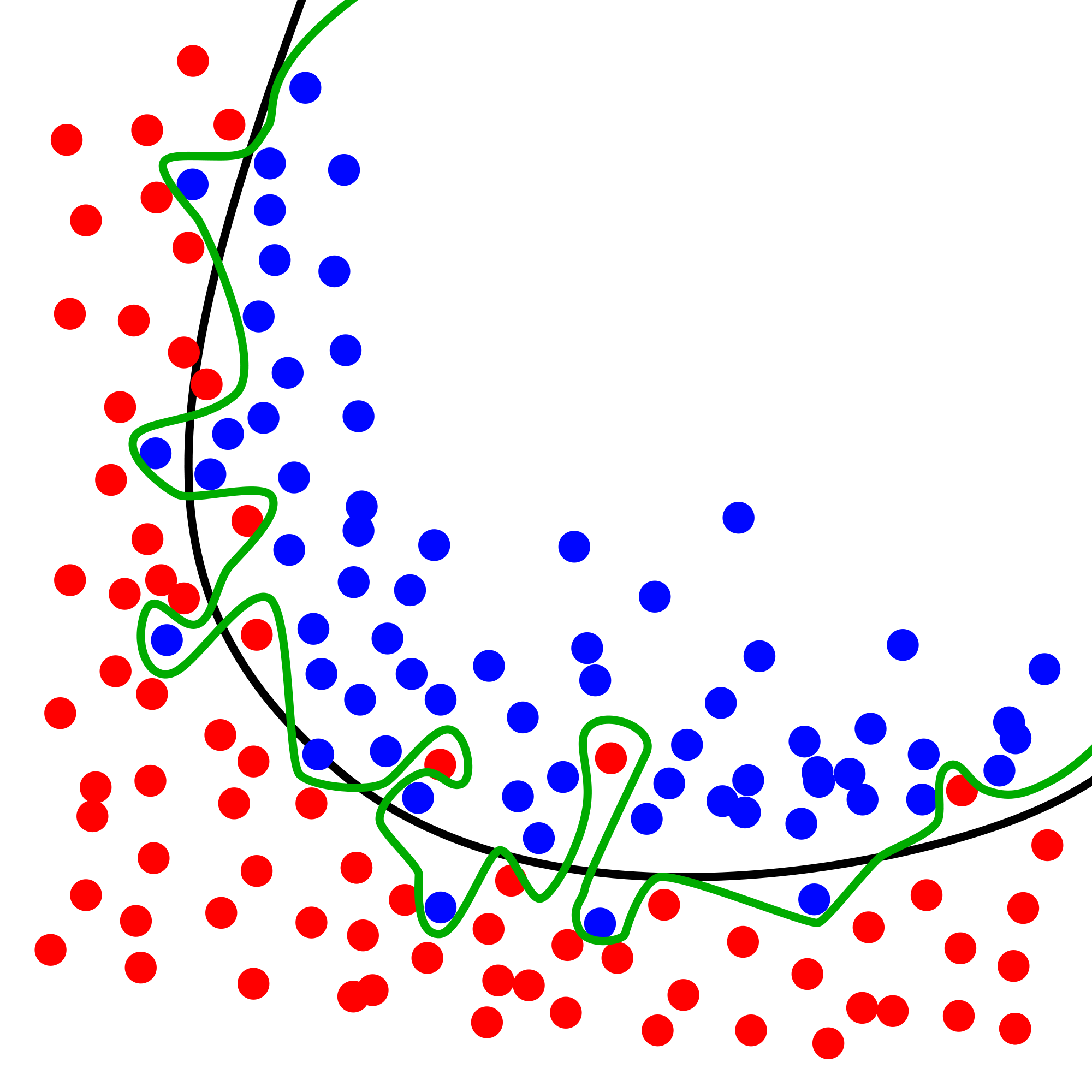
Solutions include:
- Regularization by adding a penalty to the loss function
- Early stopping
- Increase depth (more layers) and decrease breadth (less neurons per layer) leading to less parameters overall (but this creates vanishing and exploding gradient problems)
- Neural architectures adapted to the type of data leading to fewer and shared parameters (e.g. convolutional neural network or recurrent neural network)
ML implementation tools
The most popular machine learning libraries are PyTorch, developed by Facebook’s AI Research lab and TensorFlow, developed by the Google Brain Team. Both of them can be used through their Python API or through APIs in other languages.
Julia’s syntax is well suited for the implementation of mathematical models, GPU kernels can be written directly in Julia, and Julia’s speed is attractive in computation hungry fields. So Julia has also seen the development of many ML packages.
With the growing popularity of machine learning, many other packages and tools are being developed in various languages.