Zoom Our NN to classify the MNIST

Last updated: January 4, 2023

Zoom session 3 — part 1

Time: 3 pm Pacific Time.
Topic: In this session, we will build our own NN to classify the MNIST.

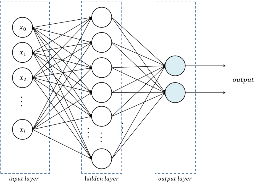
Let's build an MLP

The multi-layer perceptron (MLP) is the simplest neural network. It is a feed-forward (i.e. no loop), fully-connected (i.e. each neuron of one layer is connected to all the neurons of the adjacent layers) neural network with a single hidden layer.

Load packages

import torch
import torch.nn as nn
import torch.nn.functional as F
import torch.optim as optim
from torch.utils.tensorboard import SummaryWriter
from torchvision import datasets, transforms
from torch.optim.lr_scheduler import StepLR

The torch.nn.functional module contains all the functions of the torch.nn package.
These functions include loss functions, activation functions, pooling functions…

Create a `SummaryWriter` instance for TensorBoard

writer = SummaryWriter()

Define the architecture of the network

# To build a model, create a subclass of torch.nn.Module:
class Net(nn.Module):
	def __init__(self):
		super(Net, self).__init__()
		self.fc1 = nn.Linear(784, 128)
		self.fc2 = nn.Linear(128, 10)

    # Method for the forward pass:
	def forward(self, x):
		x = torch.flatten(x, 1)
		x = self.fc1(x)
		x = F.relu(x)
		x = self.fc2(x)
		output = F.log_softmax(x, dim=1)
		return output

Python’s class inheritance gives our subclass all the functionality of torch.nn.Module while allowing us to customize it.

Define a training function

def train(model, device, train_loader, optimizer, epoch):
    model.train()
    for batch_idx, (data, target) in enumerate(train_loader):
        data, target = data.to(device), target.to(device)
        optimizer.zero_grad()  # reset the gradients to 0
        output = model(data)
        loss = F.nll_loss(output, target)  # negative log likelihood
        writer.add_scalar("Loss/train", loss, epoch)
        loss.backward()
        optimizer.step()
        if batch_idx % 10 == 0:
            print('Train Epoch: {} [{}/{} ({:.0f}%)]\tLoss: {:.6f}'.format(
                epoch, batch_idx * len(data), len(train_loader.dataset),
                100. * batch_idx / len(train_loader), loss.item()))

Define a testing function

def test(model, device, test_loader):
    model.eval()
    test_loss = 0
    correct = 0
    with torch.no_grad():
        for data, target in test_loader:
            data, target = data.to(device), target.to(device)
            output = model(data)
            # Sum up batch loss:
            test_loss += F.nll_loss(output, target, reduction='sum').item()
            # Get the index of the max log-probability:
            pred = output.argmax(dim=1, keepdim=True)
            correct += pred.eq(target.view_as(pred)).sum().item()

    test_loss /= len(test_loader.dataset)

    # Print a summary
    print('\nTest set: Average loss: {:.4f}, Accuracy: {}/{} ({:.0f}%)\n'.format(
        test_loss, correct, len(test_loader.dataset),
        100. * correct / len(test_loader.dataset)))

Define a function main() which runs our network

def main():
    epochs = 1
    torch.manual_seed(1)
    device = torch.device('cuda:0' if torch.cuda.is_available() else 'cpu')

    transform = transforms.Compose([
        transforms.ToTensor(),
        transforms.Normalize((0.1307,), (0.3081,))
    ])

    train_data = datasets.MNIST(
        '~/projects/def-sponsor00/data',
        train=True, download=True, transform=transform)

    test_data = datasets.MNIST(
        '~/projects/def-sponsor00/data',
        train=False, transform=transform)

    train_loader = torch.utils.data.DataLoader(train_data, batch_size=64)
    test_loader = torch.utils.data.DataLoader(test_data, batch_size=1000)
    model = Net().to(device)  # create instance of our network and send it to device
    optimizer = optim.Adadelta(model.parameters(), lr=1.0)
    scheduler = StepLR(optimizer, step_size=1, gamma=0.7)

    for epoch in range(1, epochs + 1):
        train(model, device, train_loader, optimizer, epoch)
        test(model, device, test_loader)
        scheduler.step()

Run the network

main()

Write pending events to disk and close the TensorBoard

writer.flush()
writer.close()

The code is working. Time to actually train our model!

Jupyter is a fantastic tool. It has a major downside however: when you launch a Jupyter server, you are running a job on a compute node. If you want to play for 8 hours in Jupyter, you are requesting an 8 hour job. Now, most of the time you spend on Jupyter is spent typing, running bits and pieces of code, or doing nothing at all. If you ask for GPUs, many CPUs, and lots of RAM, all of it will remain idle almost all of the time. It is a really suboptimal use of Compute Canada resources.

In addition, if you ask for lots of resources for a long time, you will have to wait a long time in the queue before they get allocated to you.

Lastly, you will go through your allocation quickly.

A much better strategy is to develop and test your code (with very little data, few epochs, etc.) in an interactive job (with salloc) or in Jupyter, then, launch an sbatch job to actually train your model. This ensures that heavy duty resources such as GPU(s) are only allocated to you when you are actually needing and using them.

Concrete example with our training cluster: this cluster only has 1 GPU. If you want to use it in Jupyter, you have to request it for your Jupyter session. This means that the entire time your Jupyter session is active, nobody else can use that GPU. While you let your session idle or do tasks that do not require a GPU, this is not a good use of resources.

Let's train and test our model

Log in the training cluster

Open a terminal and SSH to our training cluster as we saw in the first lesson.

Load necessary modules

First, we need to load the Python and CUDA modules. This is done with the Lmod tool through the module command. Here are some key Lmod commands:

# Get help on the module command
$ module help

# List modules that are already loaded
$ module list

# See which modules are available for a tool
$ module avail <tool>

# Load a module
$ module load <module>[/<version>]

Here are the modules we need:

$ module load nixpkgs/16.09 gcc/7.3.0 cuda/10.0.130 cudnn/7.6 python/3.8.2

Install Python packages

You also need the Python packages matplotlib, torch, torchvision, and tensorboard.

On Compute Canada clusters, you need to create a virtual environment in which you install packages with pip.

Do not use Anaconda
While Anaconda is a great tool on personal computers, it is not an appropriate tool when working on the Compute Canada clusters: binaries are unoptimized for those clusters and library paths are inconsistent with their architecture. Anaconda installs packages in $HOME where it creates a very large number of small files. It can also create conflicts by modifying .bashrc .

For this workshop, since we all need the same packages, I already created a virtual environment that we will all use. All you have to do is to activate it with:

$ source ~/projects/def-sponsor00/env/bin/activate

If you want to exit the virtual environment, you can press Ctrl-D or run:

(env) $ deactivate

For future reference, below is how you would install packages on a real Compute Canada cluster (but please don't do it in the training cluster as it is unnecessary and would only slow it down).

Create a virtual environment:

$ virtualenv –no-download ~/env

Activate the virtual environment:

$ source ~/env/bin/activate

Update pip:

(env) $ pip install –no-index –upgrade pip

Install the packages you need in the virtual environment:

(env) $ pip install –no-cache-dir –no-index matplotlib torch torchvision tensorboard

Write a Python script

Create a directory for this project and cd into it:

mkdir mnist
cd mnist

Start a Python script with the text editor of your choice:

nano nn.py

In it, copy-paste the code we played with in Jupyter, but this time have it run for 10 epochs:

import torch
import torch.nn as nn
import torch.nn.functional as F
import torch.optim as optim
from torch.utils.tensorboard import SummaryWriter
from torchvision import datasets, transforms
from torch.optim.lr_scheduler import StepLR

writer = SummaryWriter()

class Net(nn.Module):
	def __init__(self):
		super(Net, self).__init__()
		self.fc1 = nn.Linear(784, 128)
		self.fc2 = nn.Linear(128, 10)

	def forward(self, x):
		x = torch.flatten(x, 1)
		x = self.fc1(x)
		x = F.relu(x)
		x = self.fc2(x)
		output = F.log_softmax(x, dim=1)
		return output

def train(model, device, train_loader, optimizer, epoch):
    model.train()
    for batch_idx, (data, target) in enumerate(train_loader):
        data, target = data.to(device), target.to(device)
        optimizer.zero_grad()
        output = model(data)
        loss = F.nll_loss(output, target)
        writer.add_scalar("Loss/train", loss, epoch)
        loss.backward()
        optimizer.step()
        if batch_idx % 10 == 0:
            print('Train Epoch: {} [{}/{} ({:.0f}%)]\tLoss: {:.6f}'.format(
                epoch, batch_idx * len(data), len(train_loader.dataset),
                100. * batch_idx / len(train_loader), loss.item()))

def test(model, device, test_loader):
    model.eval()
    test_loss = 0
    correct = 0
    with torch.no_grad():
        for data, target in test_loader:
            data, target = data.to(device), target.to(device)
            output = model(data)
            test_loss += F.nll_loss(output, target, reduction='sum').item()
            pred = output.argmax(dim=1, keepdim=True)
            correct += pred.eq(target.view_as(pred)).sum().item()

    test_loss /= len(test_loader.dataset)

    print('\nTest set: Average loss: {:.4f}, Accuracy: {}/{} ({:.0f}%)\n'.format(
        test_loss, correct, len(test_loader.dataset),
        100. * correct / len(test_loader.dataset)))

def main():
    epochs = 10  # don't forget to change the number of epochs
    torch.manual_seed(1)
    device = torch.device('cuda:0' if torch.cuda.is_available() else 'cpu')

    transform = transforms.Compose([
        transforms.ToTensor(),
        transforms.Normalize((0.1307,), (0.3081,))
    ])

    train_data = datasets.MNIST(
        '~/projects/def-sponsor00/data',
        train=True, download=True, transform=transform)

    test_data = datasets.MNIST(
        '~/projects/def-sponsor00/data',
        train=False, transform=transform)

    train_loader = torch.utils.data.DataLoader(train_data, batch_size=64)
    test_loader = torch.utils.data.DataLoader(test_data, batch_size=1000)
    model = Net().to(device)
    optimizer = optim.Adadelta(model.parameters(), lr=1.0)
    scheduler = StepLR(optimizer, step_size=1, gamma=0.7)

    for epoch in range(1, epochs + 1):
        train(model, device, train_loader, optimizer, epoch)
        test(model, device, test_loader)
        scheduler.step()

main()

writer.flush()
writer.close()

Write a Slurm script

Write a shell script with the text editor of your choice:

nano nn.sh

This is what you want in that script:

#!/bin/bash
#SBATCH --time=5:0
#SBATCH --cpus-per-task=1
#SBATCH --gres=gpu:1
#SBATCH --mem=4G
#SBATCH --output=%x_%j.out
#SBATCH --error=%x_%j.err

python ~/mnist/nn.py

Notes:

--time accepts these formats: "min", "min:s", "h:min:s", "d-h", "d-h:min" & "d-h:min:s"
%x will get replaced by the script name & %j by the job number

Submit a job

Finally, you need to submit your job to Slurm:

$ sbatch ~/mnist/nn.sh

You can check the status of your job with:

$ sq

PD = pending
R = running
CG = completing (Slurm is doing the closing processes)
No information = your job has finished running

You can cancel it with:

$ scancel <jobid>

Once your job has finished running, you can display efficiency measures with:

$ seff <jobid>

Let's explore our model's metrics with TensorBoard

TensorBoard is a web visualization toolkit developed by TensorFlow which can be used with PyTorch.

Because we have sent our model's metrics logs to TensorBoard as part of our code, a directory called runs with those logs was created in our ~/mnist directory.

Launch TensorBoard

TensorBoard requires too much processing power to be run on the login node. When you run long jobs, the best strategy is to launch it in the background as part of the job. This allows you to monitor your model as it is running (and cancel it if things don't look right).

Example:

#!/bin/bash
#SBATCH ...
#SBATCH ...

tensorboard --logdir=runs --host 0.0.0.0 &
python ~/mnist/nn.py

Because we only have 1 GPU and are taking turns running our jobs, we need to keep our jobs very short here. So we will launch a separate job for TensorBoard. This time, we will launch an interactive job:

salloc --time=1:0:0 --mem=2000M

To launch TensorBoard, we need to activate our Python virtual environment (TensorBoard was installed by pip):

source ~/projects/def-sponsor00/env/bin/activate

Then we can launch TensorBoard in the background:

tensorboard --logdir=~/mnist/runs --host 0.0.0.0 &

Now, we need to create a connection with SSH tunnelling between your computer and the compute note running your TensorBoard job.

Connect to TensorBoard from your computer

From a new terminal on your computer, run:

ssh -NfL localhost:6006:<hostname>:6006 userxxx@uu.c3.ca

Replace <hostname> by the name of the compute node running your salloc job. You can find it by looking at your prompt (your prompt shows <username>@<hostname>).

Replace <userxxx> by your user name.

Now, you can open a browser on your computer and access TensorBoard at http://localhost:6006.